Table of Contents
Approved
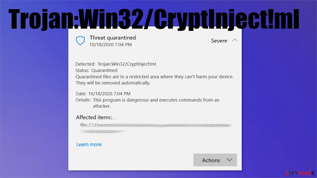
If you have win32.crypt removal on your system, this user guide should help you. Trojan Horse: Win32 / CryptInject! ml is a heuristic detection tool designed for general Trojan horse detection.
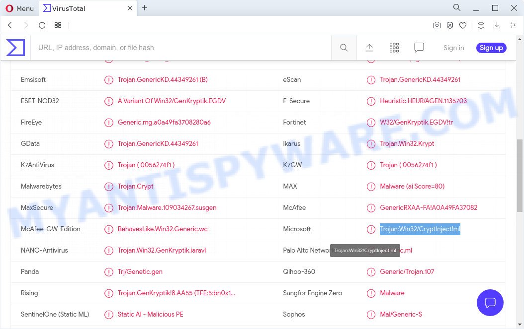
Trojan. Crypt is Malwarebytes’ generic name for detecting Trojans that experts say are obfuscated in one way or another.
completely
Today’s author, Greg Truby, Excel MVP, details some of the common problems you may encounter when using the VLOOKUP function.
In this article,A basic understanding of the VLOOKUP() function is assumed, which is one of the easiest ways to look up the value of a key in one worksheet, or provide important information from a second worksheet, and lock and lock related information directly from a worksheet. second worksheet or block. When using We vlookup() we sometimes run into three very common problems:
We need to search across multiple columns
We get a great #n/a, the key will be valid
We ran into a problem with Zoolander
Problem #1: We need to find something in a column, but we need to look up two indexes instead of one. Let’s say we might need to resend the documents in the next array.
We can’t just use the order of the colors. Will “red” mean Washington? Or Michigan? We can’t just use the entire food column, wouldn’t the “apples” be evil Washington? Or Pennsylvania? We need to search both products and colors.
Solution to problem #1. A fairly simple solution is to create a secretary that concatenates two keys once. To improve readability, we could optionally add some kind of delimiter between the two fields, such as a new (|), a comma, or a semicolon. We When we combine two or more pieces of text (which are probably often referred to as “lines of text” or simply “lines”), we call this addition process “concatenation”. The concatenation operator found by Excel is the ampersand (&), our helper formula (using the symbol TV) will beNo look like this:
After pasting the column and formula helper and copying them directly, you will get a table of results. Please note that our compound hug must always be to the left of the column from which we will return the data file.
Washington
Cherry
Red
Cherry|Red
Michigan
Bananas
Yellow
Bananas|Yellow
Hawaii
Lemons
Yellow
Lemon|Yellow
Texas
Grapes
Green
Grapes|Green readabilitydatatable=”1″>
Produce
color
Compound
Status
Apples
Red
Apples|Red
California
Apples
Green
Apples|Green
Approved
The ASR Pro repair tool is the solution for a Windows PC that's running slowly, has registry issues, or is infected with malware. This powerful and easy-to-use tool can quickly diagnose and fix your PC, increasing performance, optimizing memory, and improving security in the process. Don't suffer from a sluggish computer any longer - try ASR Pro today!

Pennsylvania
Grapes
Purple
Use Malwarebytes to remove Win32:Malware-gen virus.STEP 2: Use HitmanPro to scan for malicious unwanted programs.STEP 3: Check for malware using the Emsisoft emergency kit.STEP 4: It’s better to reset your browser settings to default.
New
Download. Download our free removal tool: rmvirut.exe.We launch the most important tool. Run the tool to remove the infected information.Update. After restarting your computer, make sure you have the latest version of your antivirus and then perform a full scan of your computer.
Grapes|York purple
We can createz corresponding composite column that can be used in most VLOOKUP() functions, or we can concatenate in a VLOOKUP() formula. Examine the formula in the formula we are going to block to see an example related to it. #2:
Problem We know our personal data matches, but the VLOOKUP() function returns #N/A.
Solution #2: The problem is almost certainly that the keys contain various numeric values and text levels in the cells, with one of the key columns formatted as GENERAL this way and the other methodically organized as TEXT. Here, the key on the left of the table is in general format, while the key on the right is in text format.
The main solution we usually come up with is definitely “I’m going to format the ‘General’ column as text” (or vice versa). .So, .select .one .of .its .columns .and .press .Ctrl+F1 .(or .Home .| .Format .| .Format .Cells .(2007, .2010) .Format .or .| . Cells… .(2003 .and .below)) .and .change .layout .and… .. This is !? decides that there is no problem. Editing a non-cell file lasts until you edit a specific cell. When we have more than a few lines, we usually don’t want to go back and press F2 after entering this value several hundred times. We have two other options. One is the built-in use of an Excel error when highlighted to find us. In the screenshot below, information technology does this. So we can select all the cells in this column and select “Convert Successful Number” in the error correction window.
If we don’t have this error correction option, or if we all just prefer the method, this is the one we can use the text-to-columns package instead. To useTo use it, we set the highlight of the column we really want to format, we want then in the exact menu (here using Excel 2007) select “Data | In text columns…” and we will also see how the master hears the following:
We can just leave the DELIMITED option in place and click and just click Next > and then make sure the delimiter being tested doesn’t appear in all of your columns. Usually the simple fact of using TAB works well because it is extremely rare in a cell. Then we click “Next”> to select a new step 3. We choose, I would say, the format we need, “General” or “Text”, and click “Finish”.
Assuming we’ve correctly specified the required format, we should be rewarded with a VLOOKUP() clause that works correctly.
An alternative solution. If we’re feeling adventurous, we can perform a type conversion on the formula, usually forcing data types. If the cells that appear to come first in the VLookup message are formatted as TEXT, and the keys that are in the entire formatted rangee in battle, the second is formatted as GENERAL, then factor as:
The software to fix your PC is just a click away - download it now.Open a new Windows Explorer window. For Windows g Server and (R2) 2008 users, click Start > Computer.In the Computer/Search on this PC field %Programs%Common:FilesSystemsymsrv enter.Once you find them, you select the file and press SHIFT+DELETE to delete it.Repeat the steps all for the presentations listed above. You
![]()
![]()
![]()
![]()
![]()
![]()
![]()
![]()
![]()
![]()